Meuse Data Example

This vignette provides examples of setting up non-spatial and spatial finite mixture models (FMMs) using clustTMB.

Fitting clustTMB models

Data Overview

The meuse data set from the sp library (Pebesma and Bivand 2005) consists of 155 observations, 4 response variables, location data, and 8 covariates. The response involves four heavy metals measured to monitor pollution levels in the top soil of the Meuse river floodplain, Netherlands (Fig. @ref(fig:sample), (Rikken and Rijn 1993)). The heavy metal data exhibit normality on the logscale (Fig. @ref(fig:pairs-expl)), allowing for a comparison between the Gaussian and lognormal distributions in addition to an FMM with and without spatial structure influencing the cluster probability.

# load data
library(sp)
data("meuse")
data("meuse.riv")
data("meuse.grid")

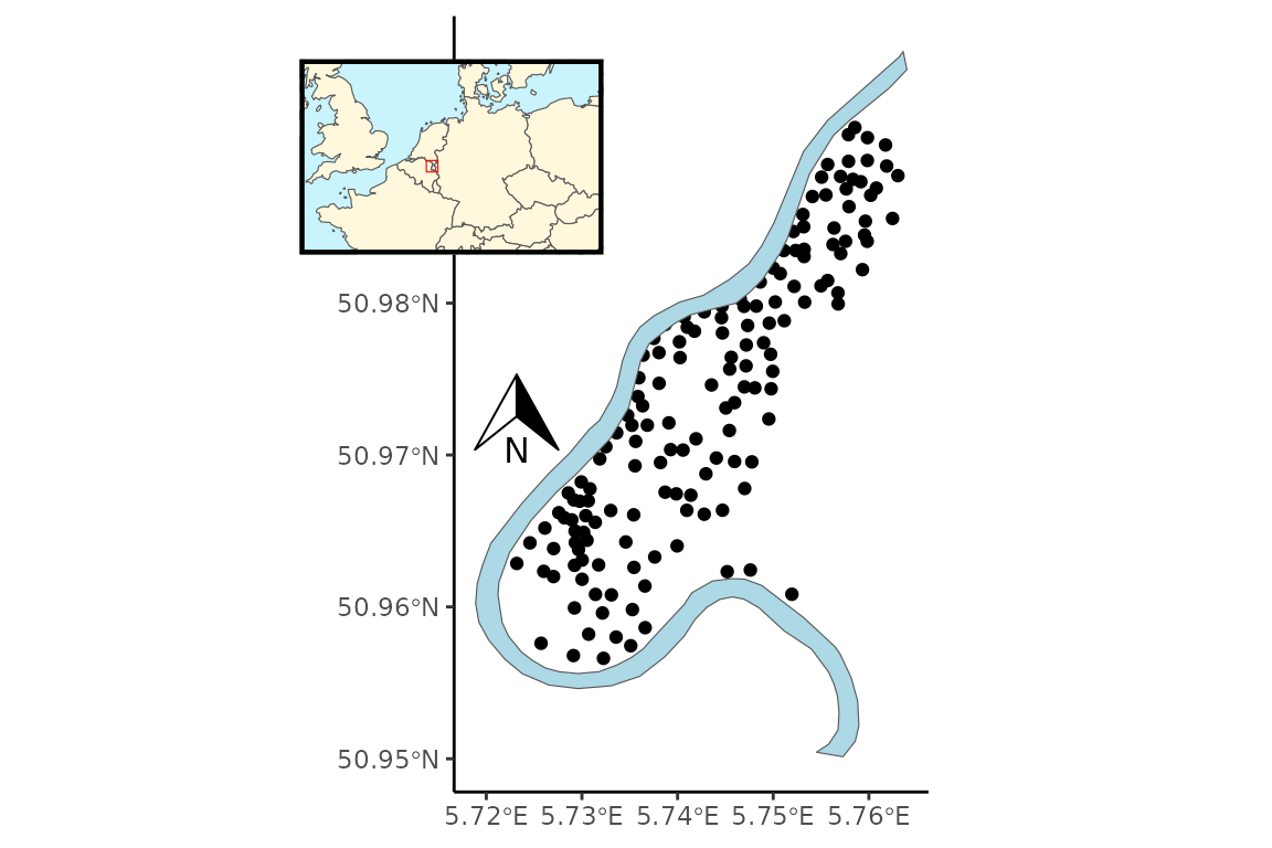
Sample locations of heavy metal concentration levels (ppm) of four metals in the topsoil of the Meuse river floodplain, Netherlands.

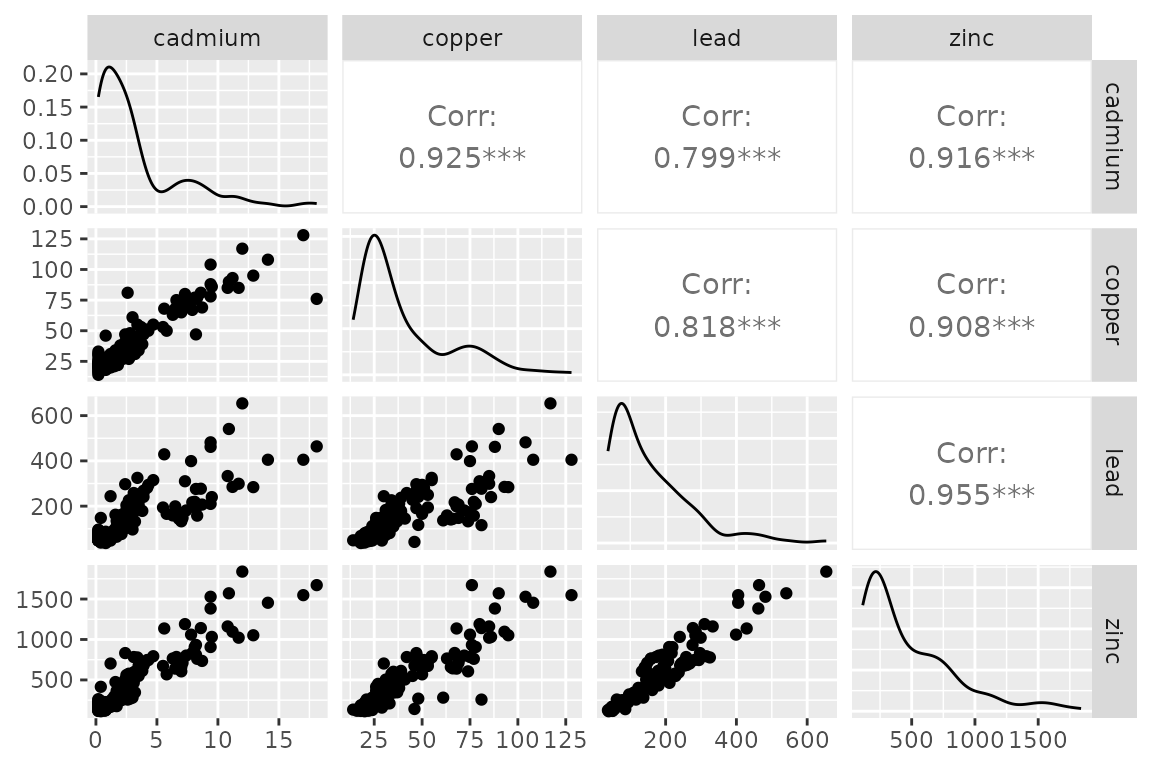
Pairs plots of the concentration levels (ppm) of four heavy metals measured in the topsoil of the Meuse river floodplain, Netherlands.

Simple FMM

The simple Gaussian FMM can be fit using the following code:

library(clustTMB)
mod.gauss <- clustTMB(response = meuse[, 3:6], G = 3, covariance.structure = "VVV")

Specifying a lognormal distribution is implemented using the family and link specification:

mod.ln <- clustTMB(
  response = meuse[, 3:6],
  family = lognormal(link = "identity"),
  G = 3, covariance.structure = "VVV"
)

Spatial FMM

The inclusion of spatial random effects in the expectation of the cluster probability in clustTMB depends on the SPDE-FEM approximation to a spatial Gaussian Markov Random Field (GMRF) introduced by the package, R-INLA. See Spatial GMRF and Gating Network for details on these clustTMB formulations. The fmesher R package (github source code) is used to run functions needed to implement this SPDE-FEM method.

Setting up the spatial mesh

The spatial model in clustTMB first requires the definition of the spatial mesh. This mesh defines the discretization of the continuous space using a constrained Delaunay triangulation. For details on building the spatial mesh, see Krainski et al., 2021, Sec 2.6.

As an example, the spatial mesh for the meuse data is built using the fmesher functions, fm_nonconvex_hull() to set up the boundary and fm_mesh_2d() to generate the spatial mesh:

library(fmesher)
loc <- meuse[, 1:2]
Bnd <- fmesher::fm_nonconvex_hull(as.matrix(loc), convex = 200)
meuse.mesh <- fmesher::fm_mesh_2d(as.matrix(loc),
  max.edge = c(300, 1000),
  boundary = Bnd
)

The inlabru R package can be used to visualize the mesh:

ggplot() +
  inlabru::gg(meuse.mesh) +
  geom_point(mapping = aes(x = loc[, 1], y = loc[, 2], size = 0.5), size = 0.5) +
  theme_classic()

## Loading required namespace: INLA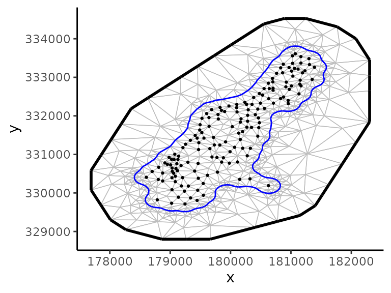

Fitting a spatial model with clustTMB

Coordinates are converted to a spatial point data frame and read into the clustTMB model, along with the mesh, using the spatial.list argument. Spatial projections can be generated by defining a spatial data frame of prediction coordinates. These can be passed into the model via the projection.dat argument of clustTMB. The gating formula is specified using the gmrf() command:

# convert coordinates to a spatial point data frame
Loc <- sf::st_as_sf(loc, coords = c("x", "y"))

# define spatial prediction coordinates
data("meuse.grid")
Meuse.Grid <- sf::st_as_sf(meuse.grid, coords = c("x", "y"))
mod.ln.sp <- clustTMB(
  response = meuse[, 3:6],
  family = lognormal(link = "identity"),
  gatingformula = ~ gmrf(0 + 1 | loc),
  G = 4, covariance.structure = "VVV",
  spatial.list = list(loc = Loc, mesh = meuse.mesh),
  projection.dat = Meuse.Grid
)

## intercept removed from gatingformula
##             when random effects specified

Results can be viewed via model output:

# Estimated fixed parameters
summary(mod.ln.sp$sdr, "fixed")

##             Estimate Std. Error
## betag      0.1778785 0.51240458
## betag      0.5710390 0.50603429
## betag      0.1653808 0.50250651
## betad      2.0157770 0.09100913
## betad      4.3160891 0.03898696
## betad      5.4259812 0.08790451
## betad      6.7095828 0.08920024
## betad      1.0064910 0.03967188
## betad      3.6030481 0.03008716
## betad      5.2113125 0.04647308
## betad      6.2155339 0.04388005
## betad      0.1259838 0.06249976
## betad      3.1475098 0.02038039
## betad      4.2016963 0.04031237
## betad      5.2523458 0.03330879
## betad     -1.4361518 0.05510443
## betad      3.1132965 0.03560883
## betad      4.2118628 0.04706053
## betad      5.1996580 0.04976699
## theta     -1.2100719 0.16013314
## theta     -2.9055373 0.19071112
## theta     -1.2794893 0.15756739
## theta     -1.2502242 0.13950032
## theta     -2.5624052 0.17078591
## theta     -3.1154930 0.13779703
## theta     -2.2459437 0.13350834
## theta     -2.3607707 0.13177544
## theta     -1.8075154 0.17469346
## theta     -4.0486948 0.19343266
## theta     -2.6845241 0.14489396
## theta     -3.0661981 0.15617972
## theta     -2.4648459 0.25661330
## theta     -3.3381189 0.23942086
## theta     -2.7804368 0.20016942
## theta     -2.6686023 0.19753757
## ln_kappag -5.9132622 0.28191115

# Minimum negative log likelihood
mod.ln.sp$opt$objective

## [1] 2318.892

Comparison Case Study

A cluster analysis was run on the meuse dataset using the Gaussian and lognormal family with and without spatial random effects in the gating network for clusters ranging from 2 to 10. BIC scores favored the lognormal spatial model with 4 clusters (Table @ref(tab:BIC)). This model resulted in fewer clusters compared to the spatial Gaussian model.

Optimum cluster size and BIC scores for lognormal and Gaussian models with (1) and without (0) spatial random effects in the gating network.

family	space	clusters	BIC
lognormal	1	4	4805
lognormal	0	4	4861
Gaussian	1	6	4861
Gaussian	0	3	4910

Results from the optimal model suggested a spatial pattern where the highest ppm observations for all four metals were clustered together (Cluster 0) in a narrow strip along the bank of the Meuse River within the northwest corner of the floodplain (Fig. @ref(fig:pairs), Fig. @ref(fig:pred)). A separate cluster (Cluster 3) was characterized by low ppm values for all metals and was spatially distributed in the central region of the floodplain. The other two clusters were characterized by moderately low (Cluster 2) and moderately high (Cluster 1) ppm values for all metals. Spatial predictions of clustered heavy metals in the Meuse River floodplain (Fig. @ref(fig:pred)) can aid in risk assessment and environmental mitigation measures after flood events.

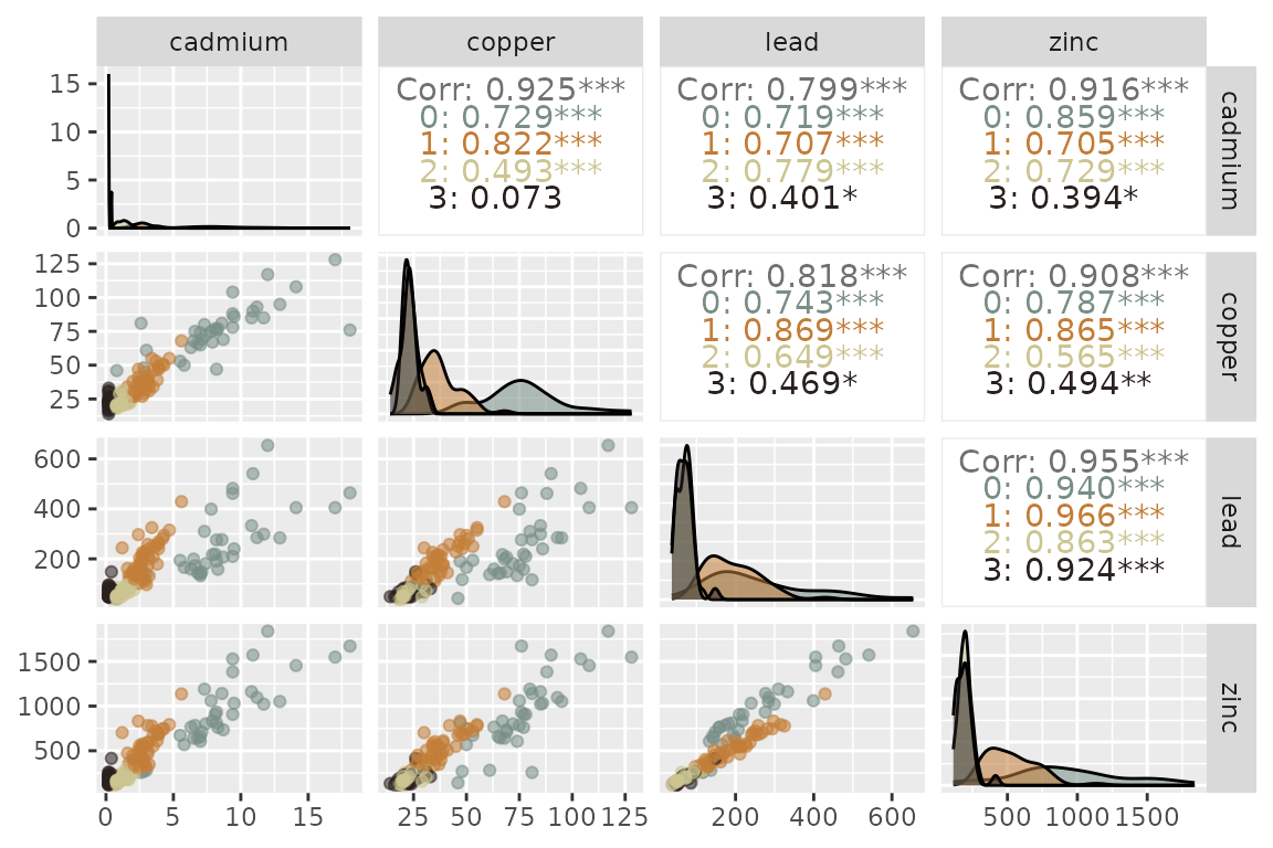
Pairs plots of the concentration levels (ppm) of four heavy metals measured in the topsoil of the Meuse river floodplain, Netherlands. Colors represent the four clusters estimated in the spatial lognormal FMM.

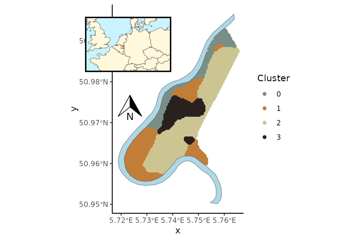
Predicted cluster distribution of heavy metal concentration levels (ppm) of four metals in the topsoil of the Meuse river floodplain, Netherlands. Colors represent the four clusters estimated in the spatial lognormal FMM.

clustTMB Formulations

Spatial GMRF

clustTMB fits spatial random effects using a Gaussian Markov Random Field (GMRF). The precision matrix, $Q$, of the GMRF is the inverse of a Matern covariance function and takes two parameters: 1) $\kappa$, which is the spatial decay parameter and a scaled function of the spatial range, $\phi = \sqrt{8}/\kappa$, the distance at which two locations are considered independent; and 2) $\tau$, which is a function of $\kappa$ and the marginal spatial variance $\sigma^{2}$:

$$\tau = \frac{1}{2\sqrt{\pi}\kappa\sigma}.$$ The precision matrix is approximated following the SPDE-FEM approach, where a constrained Delaunay triangulation network is used to discretize the spatial extent in order to determine a GMRF for a set of irregularly spaced locations, $i$. For details on the SPDE-FEM approach, see Krainski et al., 2021, Sec. 2.2

$$\omega_{i} \sim GMRF(Q[\kappa, \tau])$$

Gating Network

When random effects, $\mathbb{u}$, are specified in the gating network, the probability of cluster membership $\pi_{i,g}$ for observation $i$ is fit using multinomial regression:

$$\begin{align} \mathbb{\eta}_{,g} &= X\mathbb{\beta}_{,g} + \mathbb{u}_{,g} \\ \mathbb{\pi}_{,g} &= \frac{ exp(\mathbb{\eta}_{,g})}{\sum^{G}_{g=1}exp(\mathbb{\eta}_{,g})} \end{align}$$

References

Pebesma, Edzer J., and Roger Bivand. 2005. “Classes and Methods for Spatial Data in R.” R News 5 (2): 9–13. https://CRAN.R-project.org/doc/Rnews/.

Rikken, M. G. J., and R. P. G. van Rijn. 1993. Soil pollution with heavy metals - an inquiry into spatial variation, cost of mapping and the risk evaluation of copper, cadmium, lead and zinc in the floodplains of the Meuse west of Stein, the Netherlands. Doctoraalveldwerkverslag, Dept. of Physical Geography, Utrecht University.